What is covered?
- Overview
- Dataset
- Importing the libraries
- Loading the dataset
- Setting data shape
- One hot encoding
- Building and compiling the model
- Callbacks
- Training and visualizing the model
- Visualize model output
Overview
This post covers the development of handwritten number recognition model using MNIST dataset using Keras in Tensorflow 2.3. A step by step guide is provided to classify and recognize each digit along with the logical explanation of each line of code. I have also discussed about the basic practices that you should consider while building the model. This can also act as a skeleton to build your own classification model. You may need to go through my previous post on Overview of deep learning basics (I, II and III) before continuing here.
Dataset
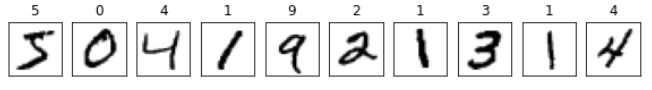
The MNIST dataset is ubiquitous with Computer Vision as it is one of the most famous computer vision challenges. The MNIST dataset was developed as the US Postal Service for automatically reading and identifying the postcodes on mail. It is a fairly large dataset that comprises of 60,000 training images and 10,000 test images of 28×28 size. Some of the sample images are shown in Fig. 1. For more details about MNIST, click here.
Importing the libraries
from tensorflow.keras import models, layers
from tensorflow.keras.datasets import mnist
from tensorflow.keras.utils import to_categorical
from tensorflow.keras.callbacks import ModelCheckpoint, TensorBoard, CSVLogger, EarlyStopping
import matplotlib.pyplot as plt
import numpy as np
import cv2
import tensorflow as tf
import datetime
import keras_metrics as km
Loading the dataset
Due to the high utility of MNIST dataset, this is one of the dataset that can directly be loaded using Keras library. You can directly load the dataset as follows:
(x_train, y_train), (x_test, y_test) = mnist.load_data()To view the sample images as shown in Fig. 1 execute following line of codes:
fig, ax = plt.subplots(1, 10, figsize=(10,10))
for i in range(0, 10):
    ax[i].xaxis.set_visible(False)
    ax[i].yaxis.set_visible(False)
    ax[i].set_title(y_train[i])
    ax[i].imshow(x_train[i], cmap=plt.cm.binary)
Getting data into shape
The current of the dataset can be viewed as below:
print('Shape of the training data, 'x_train.shape)The above line of code generates (60000, 28, 28). However, in Keras library we need to define the images in the format as follows: number of samples, width, height, depth. To attain this format:
x_train = np.expand_dims(x_train, axis=-1).astype('float32')
x_test = np.expand_dims(x_test, axis=-1).astype('float32')
x_train /= 255
x_test /= 255
The axis = -1 signifies to append the dimension at the end of current shape and .astype(‘float32’) converts the integer into the floating point and perform data normalization. Data normalization is necessary to make the training process faster and efficient.
The final shape of the dataset can be viewed as follows:
print('Data shape', x_train.shape)
print('Number of training samples:', x_train.shape[0])
print('Number of testing samples:', x_test.shape[0])
Data shape (60000, 28, 28, 1)
Number of training samples: 60000
Number of testing samples: 10000 One hot encoding
The labels (ground truth) for each image are provided in the form as follows: y_train = [0, 6, 5, 7, 3,….] having 60,000 elements. In case of multi-class classification the output labels are one hot encoded. This follows that each label is represented in the binary array of length of number of classes, where the index representing the class label is assigned number 1 and rest are 0. Therefore after one hot encoding the MNIST labels transform from (6000,) to (6000, 10) as shown below:
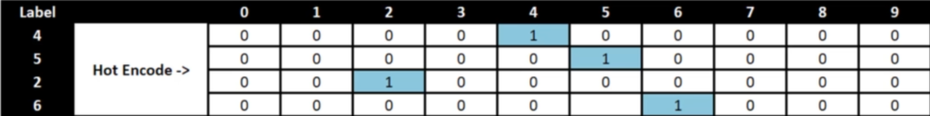
In python it can be done as follows:
y_train = to_categorical(y_train)
y_test = to_categorical(y_test)
num_classes = y_train.shape[1]
print('Number of classes: ', num_classes)
Number of classes: 10Building and compiling the model
I have build a simple CNN model that has following layers and hyperparameters:
- Input of shape: (28, 28, 1)
- This is connected to a ReLU activated convolution layer with 32 filters. The padding is kept same, this gives the output in same dimension as input. And kernel initialization is kept as He Normal. The resulting feature map is max pooled to reduce the dimension while preserving the essential high intensity features. Finally, dropout is added as a regularization.
- The step 2 is repeated with 64 filters in convolution layer.
- Another convolution layer is added with same hyperparameters. The produced feature maps are reshaped into 1 dimension (flatten()) and passed through 128 neurons. Again dropout is added as a reguarlization.
- Finally 10 neurons (number of classes) are added that generate the required probabilities at each node using softmax activation. The class is predicted based on the node with maximum probability.
model = models.Sequential()
model.add(layers.Conv2D(32, (3, 3), padding = 'same', activation='relu', kernel_initializer='he_uniform', input_shape=(x_train.shape[1], x_train.shape[2], 1)))
model.add(layers.MaxPooling2D((2, 2)))
model.add(layers.Dropout(0.25))
model.add(layers.Conv2D(64, (3, 3), padding = 'same', activation='relu', kernel_initializer='he_uniform'))
model.add(layers.MaxPooling2D((2, 2)))
model.add(layers.Dropout(0.25))
model.add(layers.Conv2D(64, (3, 3), padding = 'same', activation='relu', kernel_initializer='he_uniform'))
model.add(layers.Flatten())
model.add(layers.Dense(128, activation='relu', kernel_initializer='he_uniform'))
model.add(layers.Dropout(0.5))
model.add(layers.Dense(10, activation='softmax', kernel_initializer='glorot_uniform'))
model.compile(optimizer='adam', loss='categorical_crossentropy', metrics=['accuracy'])
model.summary()
-------------------------------------------------------------------------
Layer (type) Output Shape Param #
=========================================================================
input_5 (InputLayer) [(None, 28, 28, 1)] 0
conv2d_12 (Conv2D) (None, 28, 28, 32) 320
max_pooling2d_8 (MaxPooling2 (None, 14, 14, 32) 0
dropout_11 (Dropout) (None, 14, 14, 32) 0
conv2d_13 (Conv2D) (None, 14, 14, 64) 18496
max_pooling2d_9 (MaxPooling2 (None, 7, 7, 64) 0
dropout_12 (Dropout) (None, 7, 7, 64) 0
conv2d_14 (Conv2D) (None, 7, 7, 64) 36928
flatten_3 (Flatten) (None, 3136) 0
dense_6 (Dense) (None, 128) 401536
dropout_13 (Dropout) (None, 128) 0
dense_7 (Dense) (None, 10) 1290
-------------------------------------------------------------------------
Total params: 458,570
Trainable params: 458,570
Non-trainable params: 0The model will be trained with the categorical cross entropy function and will be evaluated using accuracy (you can add more metrics if needed) and loss values.
Callbacks
To monitor and record the performance of the model for each iteration or epoch, we will be adding certain callbacks as follows:
log_path = 'logs/'
keyname = 'mnist'
cur_date = datetime.datetime.now().strftime("%Y%m%d-%H%M%S")
tb_log_dir = log_path + "fit/" + keyname + '' + cur_date
tensorboard_callback = TensorBoard(log_dir=tb_log_dir, histogram_freq=1) model_checkpoint = ModelCheckpoint('model'+keyname+'.hdf5', monitor='loss',verbose=1, save_best_only=True)
early_stopping = EarlyStopping(monitor='val_loss', verbose=1, patience=6)
csv_logger = CSVLogger(log_path + keyname + '_' + cur_date + '.log', separator=',', append=False)
Tensorboard is used to visualize the training process in real time, ModelCheckpoint is used to save the best model weights that achieved minimal error during training and CSVLogger is used to store the metrics value for each epoch in a separate csv file. Since it is difficult to set the number of training epochs and keeping certainly large number of epochs can lead to overfitting, we need to limit the training as soon as it stops improving the results. This can be achieved by using EarlyStopping. Following this we can keep the epochs very large and stop the training process whenever loss function stops to decrease (you can choose any metric to monitor for early stopping, here we have used val_loss). The patience value indicate that window size for which to monitor validation loss, so if validation loss stops to decrease for next 6 epochs then training will halt.
Training and visualizing the model
You can start the training process as follows:
batch_size = 32
epochs = 100
val_split = 0.3
history = model.fit(x=x_train,
    y=y_train,
    batch_size=batch_size,
    epochs=epochs,
    verbose=1,
    callbacks=[model_checkpoint,early_stopping,csv_logger,tensorboard_callback],
    validation_split=val_split)
Batch size is kept 32, epochs is set to 100 and validation split is kept 30% (training data is split into 70% train data and 30% validation data). In my case the training process ends at 20th epoch with training loss and accuracy as .0218 and .9934 respectively, and validation loss and accuracy as .0371 and .9917 respectively.
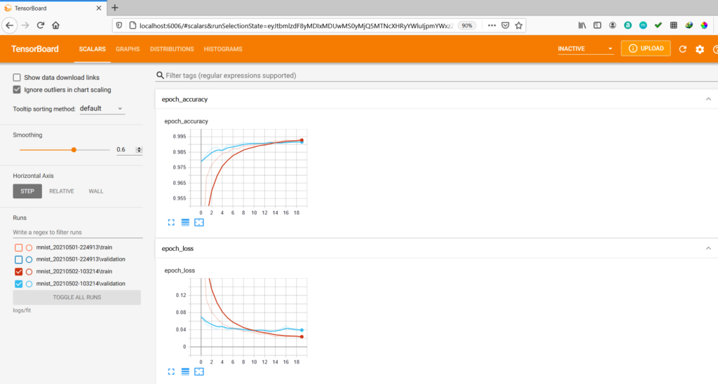
You can visualize the training progress by running following command in your command prompt with present working directory (PWD).
(tensorflow383) PWD>tensorboard --logdir logs/fit
2021-05-02 10:34:11.778801: I tensorflow/stream_executor/platform/default/dso_loader.cc:48] Successfully opened dynamic library cudart64_101.dll
Serving TensorBoard on localhost; to expose to the network, use a proxy or pass --bind_all
TensorBoard 2.3.0 at http://localhost:6006/ (Press CTRL+C to quit)
Then open the link (http://localhost:6006/) given in the command prompt in browser to visualize the metrics for each epoch.
Now the trained model can be used to evaluate its performance on the test set as follows:
score = model.evaluate(x_test, y_test)
print("Test loss: ", score[0])
print("Test accuracy: ",score[1])
313/313 [==============================] - 1s 2ms/step - loss: 0.0263 - accuracy: 0.9934
Test loss: 0.026308776810765266
Test accuracy: 0.993399977684021To predict the class for a handwritten digit you can do as follows:
idx=0
np.argmax(model.predict(np.expand_dims(x_test[idx],axis=0)), axis=-1)[0]
You can change the value of idx to predict the label for different images.
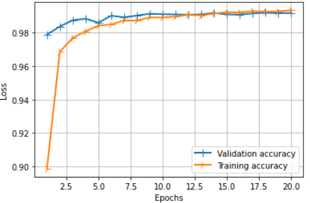
If you want to visualize the training and validation curves in python (shown in Fig. 3 and Fig. 4) then you can do as follows:
history_dict = history.history
loss_values = history_dict['loss']
val_loss_values = history_dict['val_loss']
acc_values = history_dict['accuracy']
val_acc_values = history_dict['val_accuracy']
epochs = range(1, len(loss_values) + 1)

plt.figure(figsize=(12, 3), dpi=80)
plt.subplot(1,2,1)
line1 = plt.plot(epochs, val_loss_values, label='Validation loss')
line2 = plt.plot(epochs, loss_values, label='Training loss')
plt.setp(line1, linewidth=2.0, marker = '+', markersize=10.0)
plt.setp(line2, linewidth=2.0, marker = '4', markersize=10.0)
plt.xlabel('Epochs')
plt.ylabel('Loss')
plt.grid(True)
plt.legend()
plt.show()

plt.figure(figsize=(12, 3), dpi=80)
plt.subplot(1,2,2)
line3 = plt.plot(epochs, val_acc_values, label='Validation accuracy')
line4 = plt.plot(epochs, acc_values, label='Training accuracy')
plt.setp(line3, linewidth=2.0, marker = '+', markersize=10.0)
plt.setp(line4, linewidth=2.0, marker = '4', markersize=10.0)
plt.xlabel('Epochs')
plt.ylabel('Loss')
plt.grid(True)
plt.legend()
plt.show()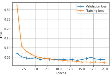
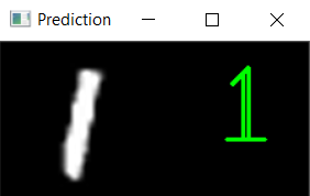
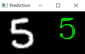
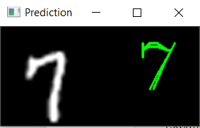
Visualize model output
The output of the model for some images can visualized as follows:
def draw_test(name, pred, input_im):
    BLACK = [0,0,0]
    expanded_image = cv2.copyMakeBorder(input_im, 0, 0, 0, input_im.shape[0], cv2.BORDER_CONSTANT, value=BLACK)
    expanded_image = cv2.cvtColor(expanded_image, cv2.COLOR_GRAY2BGR)
    cv2.putText(expanded_image, str(pred), (152, 70), cv2.FONT_HERSHEY_COMPLEX_SMALL,4,(0,255,0),2)
    cv2.imshow(name, expanded_image)
for i in range(0,10):
    rand = np.random.randint(0,len(x_test))
    input_im = x_test[rand]
    imageL = cv2.resize(input_im, None, fx=4, fy=4, interpolation=cv2.INTER_CUBIC)
    input_im = input_im.reshape(1,28,28,1)
    res = str(model.predict_classes(input_im, 1, verbose=0)[0])
    draw_test('Prediction', res, imageL)
    cv2.waitKey(0)
 cv2.destroyAllWindows()
The sample output is shown in below figures.