Overview of Deep Learning Basics - I - Punn's Deep Learning Blog

What is covered?

Introduction
Perceptron
Neural network
Activation function
Loss function
Gradient descent
Summary
Recommended resources

Prologue

Deep learning is a form of machine learning that uses a model of computing that mimics the structure of the brain, thereby calling it as Artificial Neural Network (ANN). The unprecedented success of deep learning is due to the advancements in the computing hardware i.e. Central Processing Units (CPU), Graphical Processing Units (GPU), memory and storage. Other then this, deep learning algorithms seek good quality and quantity of data which which is now widely available with vast amount of open sources.

Before diving into the ANN let’s first discuss about basic building block of the complex neural networks, an artificial neuron, known as Perceptron.

Perceptron

In biological neuron the electrical signal gets passed through the dendrites to the body of the cell and then a single output or a single electrical signal is passed via axon to other neurons. In the similar manner, we attempt to mimic this behavior into the artificial neuron (perceptron) having inputs and outputs.

For instance consider a perceptron given in Fig. 1(b) as a toy example:

We have two inputs, “Input 0” and “Input 1” and a single “Output”. The inputs can have values of features corresponding to some data or application. For now just consider 12 and 4 as some arbitrary number choices for input 0 and input 1.
The next step is to have these inputs multiplied by their respective weights represented as “Weight 0” and “Weight 1”. The weights are initialized and updated during the training process to generate the desired output. In this case we can assume the weights as 0.5 and negative 1. (Again these numbers are just arbitrary to understand the general process.)
The inputs features are multiplied by the corresponding weights. After multiplying we get 6 and negative 4.
These results are then passed into an activation function (discussed in later section. There are many activation functions to choose from. For now we will consider very simple activation function is actually going to be very simple. If the sum of the inputs is positive output one and if the sum of the inputs is negative then output zero.
We also add one bias correction term to better adjust the perceptron output.
So in this example we get, 6 – 4 + 1= 3 > 0, hence Output is 1.

In generalized representation, this computation is represented by following Eq. (1).

(1) $\begin{equation*} z = \sum_{i=0}^{n}w_ix_i + b \end{equation*}$

where $i$ is the number of input features, $w$ are weights and $b$ is a bias term.
In vector form, the Eq. 1 can be represented as Eq. 2:

(2) $\begin{equation*} z = W^TX + b \end{equation*}$

where, $W = [w_1, w_2,...., w_n]$ and $X = [x_1, x_2,...., x_n]$

Note: The above expression is without the activation function.

Neural Network

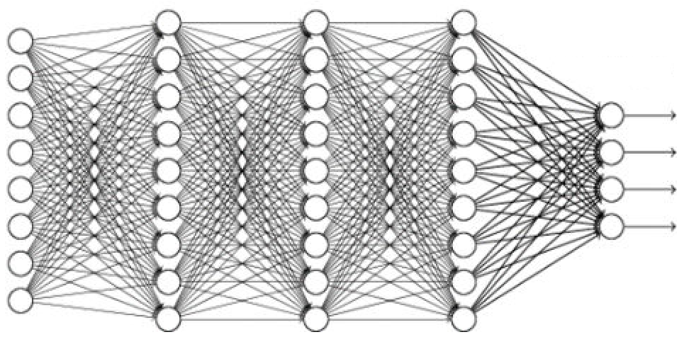
Multi-layer perceptron network – Layers of individual perceptrons are connected together through their inputs and outputs to form neural network. The sample neural network shown in Fig. 2 comprises of three types of layers:

Input layers (Purple) – fed with the features of the data.
Hidden layers (Blue and green) – layers in between input and output layers that follows complex computations to understand the hidden pattern. With high number of hidden layers the network becomes deep neural network.
Output layer (Red) – generates the desired prediction results.

Activation Function

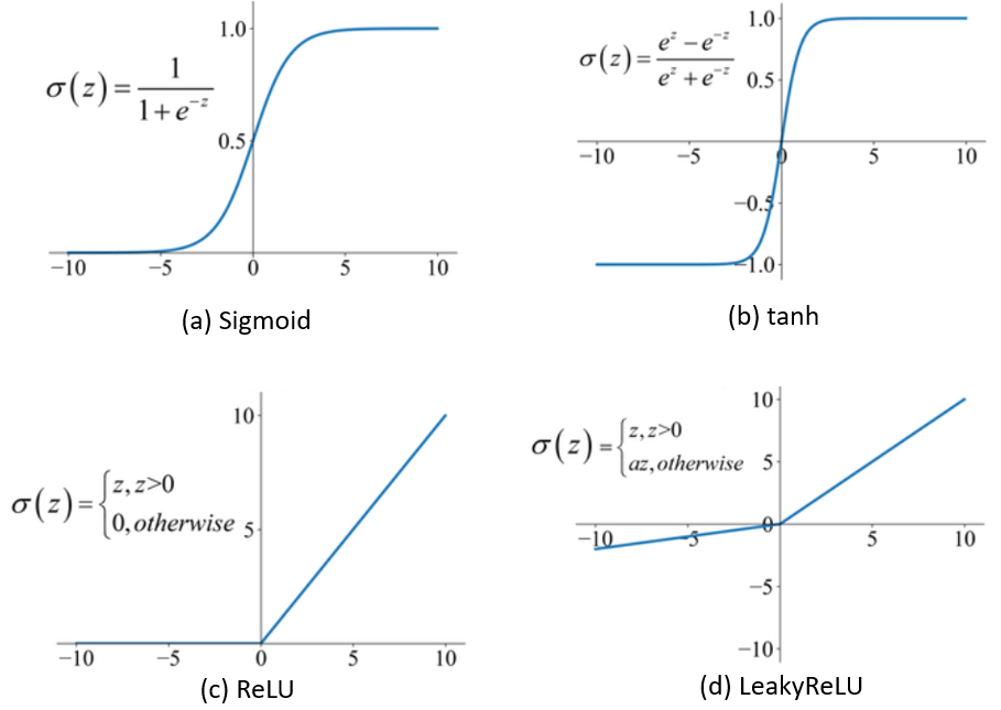
The heart of learning complex patterns lies in discovering the non-linear patterns. Activation functions are just standard normal functions that aims to add non-linearity in the output of a perceptron or any other complex computational layer. These are applied in the hidden and output layers to help network discover hidden patterns of the data. Following are the most popular activation functions that are used in neural networks:

Sigmoid function is most widely used in output layer for binary classification as its value ranges between 0 and 1. Disadvantage is that it can slow down the learning process if the value of $z$ (output of a layer) is very large or very small. Reason: slope at higher and lower value of $z$ is 0 approx. and hence when we apply gradient descent (a procedure to optimize the training parameters, $W$ ) for optimizing the loss function (variation in the prediction from the actual value), the gradient/derivatives values become very small.
tanh activation function is better than sigmoid activation function as it offers better non-linearity than sigmoid. It’s value ranges between -1 and 1. Actually, it is the scaled version of sigmoid function represented as $2\sigma (2z)$ $-1$ . So we can easily replace sigmoid with tanh and get good performance. Use of sigmoid only makes sense in the output layer and that too when we are doing binary classification i.e. the output values are 0 or 1.
ReLU it is most widely used activation function as it offers better gradients even for large values of $z$ and thus not affecting the learning rate of the model.
And Leaky ReLU is just the extension of ReLU function where for negative values of $z$ the gradient or slope is not zero. But in practice the performance is not very much affected, thereby ReLU is most widely used activation function.

Bekir Karlik and A Vehbi Olgac. 2011. Performance analysis of various activation functions in generalized MLP architectures of neural networks. International Journal of Artificial Intelligence and Expert Systems 1, 4 (2011), 111–122.
More details about the activation functions can be accessed from the above paper. Here is the link.

Cost/Loss Function

The Loss/Error/Cost/Objective functions drive the training procedure of the deep learning models. In general, you can think that the absolute difference between the predicted value ( $\hat{y}$ ) and ground truth value (actual value, $y$ ) is the error. Based on this, the squared loss function can be defined as in Eq. 3. However, due to the square factor the larger errors are more prominent and hence resulting in slowing the learning speed.

(3) $\begin{equation*} \mathcal{L} = \frac{\sum (\hat{y} - y)^2}{n} \end{equation*}$

In practice, apart from the function simplicity we also need to consider the faster convergence of the function towards global minima (achieve minimum loss value faster). Therefore, we make use of cross entropy (more details can be found here) function which is defined over the prediction probabilities, as shown in Eq. 4

(4) $\begin{equation*} \mathcal{L} = - \sum_x p(x).\log{q(x)} \end{equation*}$

where p(x) is probability of the presence of class x in the actual value and q(x) is predicted probability of the presence of class x in the final output.

There are various other loss functions to explore which are utilized based on the task or application being handled by your deep learning model. Many popular loss functions are discussed here.

Gradient Descent

It is an optimization algorithm for finding the minimum of a function (particularly error function). To find local minimum, we take steps proportional to the negative of the gradient. Meaning we take steps opposite to the direction of the gradient.

For example:

An example demonstrating gradient descent

Consider this simple example in 1 dimension. Cost on y -axis which is the result of choosing some w given on x axis.
In beginning we choose some random weight for training. Now we need to find the value of w for which the L is minimum.
We find the value of gradient or derivative at that point and see which way it goes in the negative direction.
Step by step we descent along the gradient until we get the minimum cost.

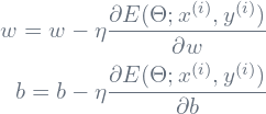
Mathematically, gradient descent can be represented as follows:

$w := w - \alpha \frac{\partial \mathcal{L}}{\partial w}$

$b := b - \alpha \frac{\partial \mathcal{L}}{\partial b}$

The above set of equations are continuously executed, where we update w and b for each epoch until global minimum is achieved i.e. the loss is minimized.

This is just a baseline approach. Now more extensions have been introduced (which can be found here – this is one of the best post about gradient descent variants – highly recommended to go through). Most popular till date is Adaptive Moment Estimation (Adam) approach to optimize the loss function.

Summary

Deep learning refers to a neural network that mimics the working of a human brain with multiple layers of linear/nonlinear processing modules. Each successive layer utilizes the output from the last layer as input to extract the complex hierarchy of features from the input data. Initiating from the multi-layer perceptron network (MLP), which forms the basis of the state-of-the-art deep learning models, comprises of a certain number of perceptrons (mathematical model of a biological neuron) with activation function, $\mathcal{F}_a$ and training parameters, $\Theta \in {\mathcal{W},\mathcal{B}}$ with $\mathcal{W}$ and $\mathcal{B}$ as set of weights ( $w$ ) and biases ( $b$ ). A typical mathematical formulation of the MLP with respect to dataset, $D\in (x_N,y_C)$ (where $x$ is the input sample, $y$ is the corresponding label, $N$ is the number of samples and $C$ is the number of classes) is represented as a linear combination of the input with training parameters followed by the activation function (sigmoid, tanh, ReLU, etc.), as shown in Eq.5. Finally, the last layer follows from the learned features to generate binary or multi-class output with certain probabilities corresponding to each class (output vector length is equal to the number of classes) following from the softmax activation function as shown in Eq.6.

(5) $\begin{equation*}\mathcal{F}_o(x;\Theta) = \mathcal{F}_a\left(w^T\mathcal{F}_a\left(w^T … \mathcal{F}_a\left(w^Tx+b\right)\right)+b\right)}\end{equation*}$

(6) $\begin{equation*}\mathcal{P}_i(\mathcal{F}_o)=\frac{e^{w^{T}_{i}x+b}}{\sum_{c=0}^{C}e^{w^{T}_{c}x+b}}\end{equation*}$

where $\mathcal{P}_i$ is the probability in the output vector corresponding to the $i^{th}$ class and $C$ indicates total number of classes.

Later, the obtained probability vector is compared with the ground truth and accordingly, the error is computed to fine-tune the training parameters and reduce the error. In case of BIS, binary cross entropy (binary class) and categorical cross entropy (multi-class) are the most popular choices as an objective function (error function, $E$ ), and are optimized with stochastic gradient descent approach. Besides, if the number of classes is two, then the categorical class entropy function (as shown in Eq.7) converges to binary cross entropy function. Finally, this error is utilized to update weights and bias values simultaneously for each training sample ( $x^{(i)}, y^{(i)}$ ) using the Eq.8, where $w$ and $b$ can be initialized using Xavier’s initializationor using the pre-trained weights, $\eta$ is the learning rate coefficient that controls the amount of deviation from the previous values by using the error gradient ( $\partial E$ ) with respect to $w$ and $b$ .

(7) $\begin{equation*}E(\Theta)=-\frac{1}{N}\left(\sum_{i=1}^{N}\sum_{c=1}^{C}1_{y_i \in C_c}\log{\mathcal{P}_i \in C_c}\right) \end{equation*}$

where the term $1{y_i \in C_c}$ indicates that $i^{th}$ observation belongs to the $c^{th}$ category and $\mathcal{P}_i \in C_c$ is the predicted probability vector of the $i^{th}$ observation that belongs the to the $c^{th}$ category.

(8) $\begin{equation*}\begin{aligned}w=w - \eta\frac{\partial E(\Theta ;x^{(i)}, y^{(i)})}{\partial w} \\b=b - \eta\frac{\partial E(\Theta ;x^{(i)}, y^{(i)})}{\partial b}\end{aligned}\end{equation*}$