Overview of Deep Learning Basics - III - Punn's Deep Learning Blog

What is covered?

Overfitting and underfitting
Regularization
Dropout
Vanishing and exploding gradient
Weights intialization

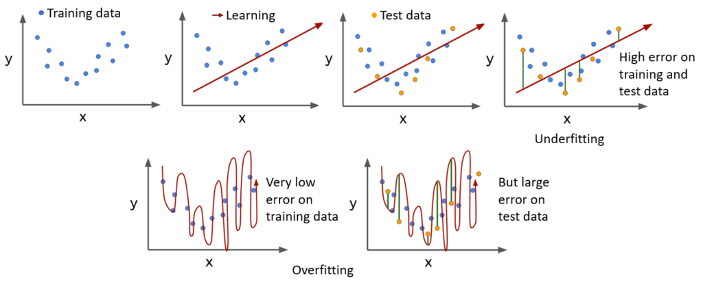
Overfitting and underfitting

During training, a neural network undergoes many epochs (may be more than 100 or 500) to learn the desired objective using the big datasets. However, most likely the neural network will learn to replicate the training data. This is very intuitive as the network trains over and over the same training datasets so many times that the neural network is going to adjust weights and biases in order to replicate 100 % as much as it can the training data.

Although this may sound good at first, however it is very problematic because the whole point of neural networks is to make predictions using never before seen data. And since it is just learned to replicate the training data, it performs poorly on the unseen test data.

Whereas, in underfitting the model fails to adapt or learn neither the training data nor the testing data. Therefore, the underfit model is not suitable to perform the desired task. The model is tends to underfit when model performs poorly on the training data.

With potentially hundreds of parameters in a deep learning neural network, the possibility of overfitting is very high.

The overfitting and underfitting will become more clear from Fig. 1. More details can be found here.

Regularization

It is generally used to prevent overfitting and is common to various machine learning problems (not unique to neural networks).
Adds a penalty for larger weights in the model.
This regularization can be expressed as Eq. 1:

(1) $\begin{equation*} \mathcal{L}(w,b) = \mathcal{L}(w,b) + \frac{\lambda}{2n}||w||^{2}_{2} \end{equation*}$

where $\mathcal{L}(w,b)$ is any loss function like cross entropy loss, dice loss, etc., $\lambda$ is the regularization parameter, $n$ is the number of data samples and $||w||^{2}_{2}$ is a term of $L_2$ regularization as shown in Eq. 2.

(2) $\begin{equation*} ||w||^{2}_{2} = \sum _{i=1}^{n}w_{i}^{2} = w^Tw \end{equation*}$

How it prevents overfitting?

If $\lambda$ is large, weights will be relatively smaller as they are penalized for increasing the loss. Which means zeroing out the impact of hidden units and deep network will become linear.

For very large values of lambda, the model moves from overfitting scenario to underfitting. So selection of some intermediate value of $\lambda$ will help prevent underfitting problem.

More details can be found here.

Dropout

Dropout is a technique to avoid overfitting in neural networks. In this we remove the neurons (restricting a neuron from sending or receiving the activations) during training randomly due to which the network does not rely on any particular neuron to identify certain pattern, thereby preventing overfitting. Researches have shown better performance in the neural networks when using dropout.

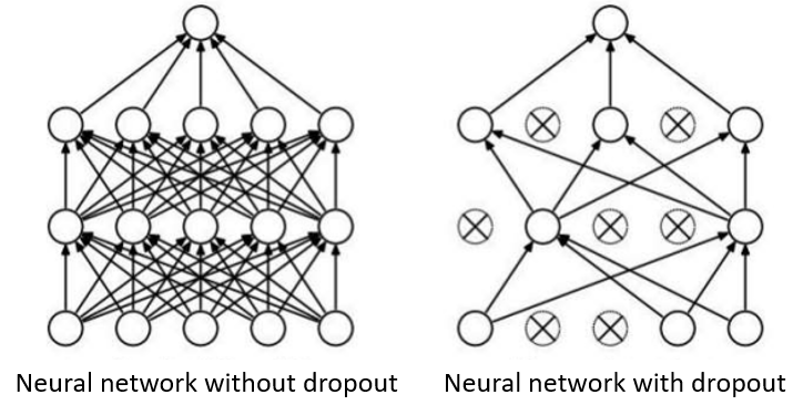
In dropout each neuron is assigned some probability (randomness) to stay active or non-active. The active nodes remain connected in the network, whereas all the incoming and outgoing connections are removed for non-active node. This results is a very much diminished network (as shown in Fig. 2) which is trained to learn a data sample. And then on another sample the probabilities are redefined and keep different set of nodes active . So for each training sample diminished networks are created, which are trained.

Note: Dropout layers are only created during training. During test time we apply no dropout. This is because when doing predictions you don’t your network to produce random output.

Vanishing and exploding gradient

When training very deep neural network, derivatives or gradients may become very small or very large. Due to which the model struggles to achieve global minima with the objective function.

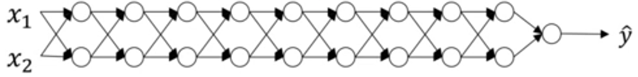
Consider a deep neural network with $l$ layers (as shown in Fig. 3) with parameters at each layer represented as $w^{[1]}, w^{[2]}, ..., w^{[l]}$ . For simplicity consider the following:

Linear activation, i.e. $\sigma(z)=z$ .
No bias, i.e. $b^{[l]}=0$

Therefore output, $\hat{y}=w^{[l]}w^{[l-1]}....w^{[2]}w^{[1]}.X$

If $w^{[l]}=\begin{bmatrix} 0.9 & 0 \\ 0 & 0.9 \end{bmatrix}$ (except for the last layer because it has different dimensions), $\hat{y}=w^{[l]}\begin{bmatrix} 0.9 & 0 \\ 0 & 0.9 \end{bmatrix}^{l-1}X$ , and hence for very deep neural network (large value of $l$ ) the value of $\hat{y}$ will vanish.

Conversely, if $w^{[l]}=\begin{bmatrix} 1.1 & 0 \\ 0 & 1.1 \end{bmatrix}$ , $\hat{y}=w^{[l]}\begin{bmatrix} 1.1 & 0 \\ 0 & 1.1 \end{bmatrix}^{l-1}X$ , and hence for very deep neural network the value of $\hat{y}$ will explode.

Therefore, we can say that if $w < I$ ( $I$ is identity matrix), for very deep network the gradients will vanish, whereas if $w > I$ , for very deep network the gradients will explode.

This problem is partially tackled by carefully initializing the weights.

Weights initialization

Zero initialization:
- No randomness in weights.
- The model behaves like a linear model because the hidden layers become symmetric.
- Not a good choice.
Random initialization:
- Better than zero initialization but not optimal.
- If randomly initialized weights are high, and considering the ReLU activation (most common choice), the output will be high. Due to which the gradients will change very slowly and training will take a lot of time. (Exploding gradient)
- However, if randomly initialized weights are low, then output activation will be mapped to 0 and hence there will be no learning at all. (Vanishing gradient)
Xavier/Glorot initialization:
- Draw weights from distribution with zero mean and a specific variance. This is done my multiplying the randomly initialized weights with the following:
  - $Var(w)=\sqrt{\frac{1}{n_{in}}}$ , where $w$ is the initialization distribution for a neuron and $n_{in}$ is number of neurons feeding into it.
- This is most widely used in case of $tanh()$ activation.
He initialization:
- This is most widely used in case of $ReLU()$ and its variants activations.
- It just replaces the numerator in the Xavier initialization with .
  - $Var(w)=\sqrt{\frac{2}{n_{in}}}$

More details about weights initialization be found here and here.