Punn's Deep Learning Blog

What is covered?

• Overview
• Importing libraries
• Loading the MNIST dataset
• Preprocessing
• Loading the trained model
• Evaluation
• Model visualization
• Filter visualization
• Class activation map
• LIME
• Conclusion

Overview

Unlike machine learning models, the deep learning models lack transparency in the decision making process, where the input and output are well-presented but the processing in the hidden layers is difficult to interpret and understand, and hence these are also termed as black-box models. To better interpret these models various visualization based approaches are proposed such as activation visualization (AV), which visualizes the object (nuclei) patterns from the model perspective, filter visualization (FV), which visualizes the layerwise output of the model, local interpretable model-agnostic explanations (LIME) are generated for a particular observation by analyzing the corresponding prediction of the model.

Following from my older post (Building First CNN Model), I will use my MNIST classification model for visualization. Follow along the following sections to see how we can visualize the model.

Importing Libraries

You may need to install some of the packages if not found in your environment.

I am using tensorflow-gpu version 2.3.

For visualization I have installed: visualkeras, LIME and tf_keras_vis

Import the following libraries to get started.

from tensorflow.keras.models import Model, load_model
from tensorflow.keras.datasets import mnist
from tensorflow.keras import layers
from tensorflow.keras.utils import to_categorical
from tensorflow.keras import backend as K
import tensorflow as tf

import numpy as np
import matplotlib.pyplot as plt
import itertools

from PIL import ImageFont
from sklearn.metrics import accuracy_score, confusion_matrix
from skimage.segmentation import mark_boundaries

import visualkeras
import lime
from lime import lime_image
from tf_keras_vis.activation_maximization import ActivationMaximization

Loading the MNIST dataset

Due to the high utility of MNIST dataset, this is one of the dataset that can directly be loaded using Keras library. You can directly load the dataset as follows:

(x_train, y_train), (x_test, y_test) = mnist.load_data()

The sample images as shown in Fig. 1 can be viewed by executing following line of codes:

fig, ax = plt.subplots(1, 10, figsize=(10,10))
for i in range(0, 10):
    ax[i].xaxis.set_visible(False)
    ax[i].yaxis.set_visible(False)
    ax[i].set_title(y_train[i])
    ax[i].imshow(x_train[i], cmap=plt.cm.binary)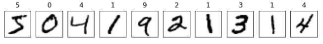

Preprocessing

The dataset needs to be preprocessed for MNIST classifier CNN model as follows:

x_train = np.expand_dims(x_train, axis=-1).astype('float32')
x_test = np.expand_dims(x_test, axis=-1).astype('float32')

x_train /= 255
x_test /= 255

print('Data shape', x_train.shape)
print('Label shape', y_train.shape)
print('Number of training samples:', x_train.shape[0])
print('Number of testing samples:', x_test.shape[0])

Data shape (60000, 28, 28, 1) 
Label shape (60000,) 
Number of training samples: 60000 
Number of testing samples: 10000

Converting the labels into one hot encoding as follows:

y_train = to_categorical(y_train)
y_test = to_categorical(y_test)
num_classes = y_train.shape[1]
num_features = x_train.shape[1] + x_train.shape[2]
print('Number of classes: ', num_classes)

Number of classes:  10

Loading the trained model

I already trained my model in my previous post. The trained model can be loaded as follows:

model = load_model('model_mnist.hdf5')
model.summary()

Model: "sequential"
_________________________________________________________________
Layer (type)                 Output Shape              Param #  
=================================================================
conv2d (Conv2D)              (None, 28, 28, 32)        320        
_________________________________________________________________ 
max_pooling2d (MaxPooling2D) (None, 14, 14, 32)        0          
_________________________________________________________________ 
dropout (Dropout)            (None, 14, 14, 32)        0          
_________________________________________________________________ 
conv2d_1 (Conv2D)            (None, 14, 14, 64)        18496      
_________________________________________________________________ 
max_pooling2d_1 (MaxPooling2 (None, 7, 7, 64)          0          
_________________________________________________________________ 
dropout_1 (Dropout)          (None, 7, 7, 64)          0          
_________________________________________________________________ 
conv2d_2 (Conv2D)            (None, 7, 7, 64)          36928      
_________________________________________________________________ 
flatten (Flatten)            (None, 3136)              0          
_________________________________________________________________ 
dense (Dense)                (None, 128)               401536     
_________________________________________________________________ 
dropout_2 (Dropout)          (None, 128)               0          
_________________________________________________________________ 
dense_1 (Dense)              (None, 10)                1290       
================================================================= 
Total params: 458,570 
Trainable params: 458,570 
Non-trainable params: 0

Evaluation

The loaded model can be evaluated as follows:

score = model.evaluate(x_test, y_test)
print("Test loss: ", score[0])
print("Test accuracy: ",score[1])

313/313 [==============================] - 0s 1ms/step - loss: 0.0263 - accuracy: 0.9934 
Test loss:  0.026308776810765266 
Test accuracy:  0.993399977684021

The confusion matrix of the classification model can be plotted as follows: (This can later be used to compute other metrics like accuracy, precision, recall, F1-score, etc.)

fig, ax = plt.subplots(1,1,figsize=(16,6.5))
shrink=1
y_pred=model.predict(x_test)
y_actual=np.argmax(y_test, axis = -1)
y_pred=np.argmax(y_pred, axis = -1)

cm = confusion_matrix(y_actual,y_pred)
cm0 = cm
cm = 100*cm.astype('float') / cm.sum(axis = 1)[:, np.newaxis]
n_classes = len((y_train[0]))
plt.sca(ax)
plt.imshow(cm, cmap = 'YlOrRd')
plt.title('Normalized confusion matrix (%)')
plt.colorbar(shrink=shrink)
tick_marks = np.arange(n_classes)
plt.xticks(tick_marks, np.arange(n_classes))
plt.yticks(tick_marks, np.arange(n_classes))
thresh = cm.max() / 2.
for i, j in itertools.product(range(cm.shape[0]), range(cm.shape[1])):
    if i!=j:
        plt.text(j, i, format(cm[i, j], '.2f'),
                 horizontalalignment="center",
                 color="white" if cm[i, j] > thresh else "black")
    if i==j:
        plt.text(j, i, format(cm[i, j], '.2f'),
                 horizontalalignment="center",
                 color="white")
plt.tight_layout()
plt.ylabel('True label')
plt.xlabel('Predicted label')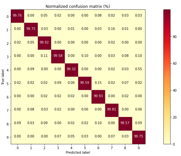

Model visualization

The overall schematic representation of the model can be viewed as shown in Fig. 2

font = ImageFont.truetype("arial.ttf", 12)
visualkeras.layered_view(model, legend=True, font=font).show()

Filter visualization

This technique highlights what pattern each layer of the model understands. Low-level filters (i.e., Conv. layers) at the beginning of a network learn low-level features, whereas high-level filters learn larger spatial patterns. Since CNNs are the representations of the visual concepts, FV helps conceptualize what the model has learned by visualizing the two-dimensional filters learned by the model and discover the types of features detected at each layer of the model

To visualize the output of the of the individual layers, say convolution layer or dense layer we can proceed as follows:

First we will see what layers are available and then select the index of the layers whose output we want to visualize. I have saved the ouput layers that I want to see in “layer_output2”.

layer_outputs = [layer.output for layer in model.layers[:]] 
for i in range(len(layer_outputs)):
    print('{} layer: {}'.format(i, layer_outputs[i]))
idx = [0, 3, 6]
layer_outputs2 = []
for temp in idx:
    layer_outputs2.append(layer_outputs[temp])

0 layer: Tensor("conv2d/Relu:0", shape=(None, 28, 28, 32), dtype=float32) 
1 layer: Tensor("max_pooling2d/MaxPool:0", shape=(None, 14, 14, 32), dtype=float32)
2 layer: Tensor("dropout/cond/Identity:0", shape=(None, 14, 14, 32), dtype=float32) 
3 layer: Tensor("conv2d_1/Relu:0", shape=(None, 14, 14, 64), dtype=float32) 
4 layer: Tensor("max_pooling2d_1/MaxPool:0", shape=(None, 7, 7, 64), dtype=float32) 
5 layer: Tensor("dropout_1/cond/Identity:0", shape=(None, 7, 7, 64), dtype=float32) 
6 layer: Tensor("conv2d_2/Relu:0", shape=(None, 7, 7, 64), dtype=float32) 
7 layer: Tensor("flatten/Reshape:0", shape=(None, 3136), dtype=float32) 
8 layer: Tensor("dense/Relu:0", shape=(None, 128), dtype=float32) 
9 layer: Tensor("dropout_2/cond/Identity:0", shape=(None, 128), dtype=float32) 
10 layer: Tensor("dense_1/Softmax:0", shape=(None, 10), dtype=float32)

Create another model with the same input as the original model and output as the layers you want to visualize. Then predict the results for some image. In this code, I selected a test image of number 7 and the output results are shown in Fig. 4.

activation_model = Model(inputs=model.input, outputs=layer_outputs2)
activations = activation_model.predict(x_test[:1])

#Visualization
images_per_row = 16
for layer_name, layer_activation in zip(layer_outputs2, activations): # Displays the feature maps
    n_features = layer_activation.shape[-1] # Number of features in the feature map
    size = layer_activation.shape[1] #The feature map has shape (1, size, size, n_features).
    n_cols = n_features // images_per_row # Tiles the activation channels in this matrix
    display_grid = np.zeros((size * n_cols, images_per_row * size))
    for col in range(n_cols): # Tiles each filter into a big horizontal grid
        for row in range(images_per_row):
            channel_image = layer_activation[0, :, :, col * images_per_row + row]
            channel_image -= channel_image.mean() # Post-processes the feature to make it visually palatable
            channel_image /= channel_image.std()
            channel_image *= 64
            channel_image += 128
            channel_image = np.clip(channel_image, 0, 255).astype('uint8')
            display_grid[col * size : (col + 1) * size, row * size : (row + 1) * size] = channel_image
    scale = 1. / size
    plt.figure(figsize=(scale * display_grid.shape[1], scale * display_grid.shape[0]))
    plt.title(str(layer_name))
    plt.grid(False)
    plt.imshow(display_grid, aspect='auto', cmap='viridis')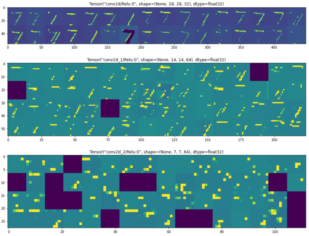

Class activation map

Class activation maps illustrate how successive layers in the model transform the input. The transformation follows from minimizing the activation maximization loss of the layer by computing its gradient w.r.t. its input and accordingly updating the input. Activation maximization loss outputs small values for large filter activation, which allows understanding input patterns activated by a particular filter.

The class activation maps can be produced as follows:

A new function is created that returns a new model with input as the original model’s input , output as the target layer (whose we want to view the activation maps) and finally we update the activation function of the output layer as linear function.

A loss function is also required that returns the arbitrary values for some filter_number (indicating the class label). This variable will be set later.

layer_name = 'dense_1' # The target layer that is kept the last layer of our model.

def model_modifier(current_model):
    target_layer = current_model.get_layer(name=layer_name)
    new_model = Model(inputs=current_model.inputs, outputs=target_layer.output)
    new_model.layers[-1].activation = tf.keras.activations.linear
    return new_model

def loss(output):
     return output[…, filter_number]

Now we can create an instance of the ActivationMaximization that takes the input as original model and a function that modifies the original model.

activation_maximization = ActivationMaximization(model, model_modifier)

The following loop generates the activation maps of the output layer for each class (shown in Fig. 5) as follows:

fig, ax = plt.subplots(1, 10, figsize=(14,14))
for i in range(0, 10):
    filter_number = i
    activation = activation_maximization(loss)
    image = activation[0].astype(np.uint8)
    ax[i].xaxis.set_visible(False)
    ax[i].yaxis.set_visible(False)
    ax[i].set_title(str(i))
    ax[i].imshow(image)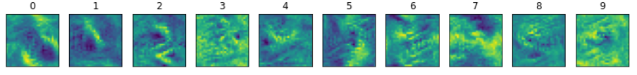

You can also try other visualizations like saliency maps, gradcam++, etc. from here.

LIME

It is a Local Interpretable Model-Agnostic Explanations technique to interpret the results of any machine learning model for a particular instance or a sample.

The procedure is as follows:

• Generate random perturbations of the instance under observation.
• Use complex model to predict the classes for new generated dataset.
• Compute the weights between the instance being explained and the each perturbation to compute weights of the generated instances.
• Use other simple model to fit new dataset with predicted value along with assigned weights.
• The feature coefficients of the simple model draws the explanation of the complex model for that instance.

To generate LIME explanations you can follow as below:

Create an instance of LimeImageExplainer.

explainer = lime_image.LimeImageExplainer()

Create a new function that produces the prediction results of an image.

def new_predict_fn(images):
    return model.predict(images[:,:,:,:1])

Generate the explanations for some instance:

explanation = explainer.explain_instance(np.squeeze(x_train[0].astype('double')), new_predict_fn, hide_color=0)
temp, mask = explanation.get_image_and_mask(explanation.top_labels[0], positive_only=True, num_features=5, hide_rest=True)
plt.imshow(mark_boundaries(temp / 2 + 0.5, mask))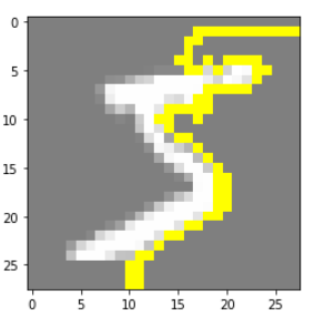

These Yellow boundary in Fig. 6 indicate the critical features that made the model to classify this image.

Conclusion

The visualization indeed are very helpful to see what model’s see and provide some understanding about why model classified the particular class. The complete source code is available on my github page here.