
Memory, State Representations, and Recurrent Neural Networks
3. Why Sequence Models Need Memory
In Part 1, sequential data was represented as an ordered collection of observations,
(3.1) 
Unlike independent data samples, observations within a sequence are temporally correlated. As discussed in Equation (2.5) of Part 1, the probability of the current observation depends on the sequence history rather than the current observation alone.
Consider a sequence model processing  one observation at a time. At time step
  , the model receives only the current observation,
  . If the model immediately discards after processing it, then when the next observation,
  arrives, no information about the previous observation remains available. Consequently, the model cannot exploit temporal dependencies that span multiple time steps.
3.1 Processing Without Memory
Suppose a model predicts an output using only the current observation. The prediction can be written as
(3.2) 
where
- denotes the current observation,
 denotes the corresponding output,
 represents the prediction function.
Equation (3.2) describes a memoryless model because the prediction depends exclusively on the current input.
Such a formulation is appropriate for independent observations such as image classification, where each image is unrelated to previous samples. However, it is inadequate for sequential data because important contextual information is ignored.
For example, consider the sentence
The bank approved the loan.
The interpretation of the word bank depends on the subsequent context. Conversely, in the sentence
The fisherman reached the bank.
the same word refers to the side of a river rather than a financial institution.
If the model processes each word independently using Equation (3.2), both occurrences of bank receive identical representations despite their different meanings.
A similar limitation arises in time-series forecasting. Predicting tomorrow’s stock price using only today’s price ignores the historical trend that often determines future market behavior.
These examples demonstrate that sequential prediction requires access to historical information.
3.2 Storing the Entire History
One straightforward solution is to retain every previous observation.
At time step , the model stores
(3.3) 
where  denotes the complete history of observations processed so far.
The prediction function now becomes
(3.4) 
Unlike Equation (3.2), Equation (3.4) has access to every previous observation in the sequence.
Although this formulation preserves all historical information, it introduces significant computational challenges.
First, the amount of stored information increases linearly with the sequence length. After processing observations, the memory requirement is proportional to . For very long sequences, such as genomic data, long documents, or continuous sensor streams, storing the complete history quickly becomes impractical.
Second, every prediction requires examining the entire history. As the sequence grows, the computational cost of accessing and processing all previous observations also increases.
Consequently, directly storing the history defined in Equation (3.3) is not a scalable solution for long-sequence modeling.
3.3 A Compact Representation of History
Instead of preserving every observation explicitly, an alternative approach is to summarize the history using a fixed-size representation.
Let
(3.5) 
denote a vector that contains all information considered relevant after processing the first observations.
Rather than storing the complete history , the model stores only the state vector  .
.
This idea can be expressed mathematically as
(3.6) 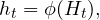
where
- denotes the complete history defined in Equation (3.3),
 denotes a function that compresses the history into a fixed-dimensional representation.
Equation (3.6) introduces one of the most fundamental concepts in sequence modeling:
The state is a compressed representation of the sequence history.
Unlike , whose size increases with the sequence length, the dimensionality of remains fixed regardless of how many observations have been processed.
For example, even if a language model processes a document containing one million words, the hidden state may still consist of only a few hundred or a few thousand numerical values.
This fixed-size representation enables sequence models to process arbitrarily long sequences while maintaining constant memory requirements for the internal state.
4. Memory as a Recursive State Representation
In the previous section, we introduced the concept of a state as a compact representation of the sequence history. Instead of storing every previous observation, the model maintains a fixed-dimensional vector that summarizes all relevant information processed so far.
Mathematically, the state was defined as
(4.1) 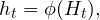
where denotes the sequence history up to time step , and is a function that compresses the history into a fixed-size representation.
Although Equation (4.1) defines what the state represents, it does not explain how the state is computed. A straightforward implementation would require recomputing the entire history every time a new observation arrives, which defeats the purpose of maintaining a compact memory.
The key insight behind modern sequence models is that the state does not need to be recomputed from scratch. Instead, it can be updated recursively.
4.1 Recursive Computation of State
Suppose the model has already processed the first  observations. At this point, it has computed the state
  , which summarizes the history
  . When the next observation, arrives, the complete history becomes
  .
.
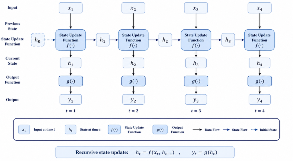
Instead of recomputing the entire history , the model only needs to incorporate the newly observed input into the existing state. This idea leads to the recursive update equation
(4.2) 
where
- is the previous state,
- is the current observation,
- is the state-update function.
Equation (4.2) is one of the most fundamental equations in sequence modeling.
Unlike Equation (4.1), which views the state as a function of the complete history, Equation (4.2) shows that the state can be updated incrementally using only two quantities:
- the previous state,
- the current input.
No earlier observations need to be stored explicitly.
4.2 Why Does the Recursive Formulation Work?
To understand why Equation (4.2) is sufficient, consider how information accumulates over time.
At time step  , the state is computed as
(4.3) 
where  denotes the initial state.
After observing the second input,  , the state becomes
(4.4) 
Substituting Equation (4.3) into Equation (4.4) gives

Similarly,
(4.5) 
which expands to

Continuing this process,

This recursive expansion reveals an important property:
Although the model stores only the current state
Consequently, the state functions as a compressed representation of the entire sequence history.
4.3 The State as a Dynamic Memory
The recursive formulation introduced in Equation (4.2) transforms the state into a dynamic memory.
At every time step, two operations are performed:
- Information from the previous state is retained.
- Information from the current observation is incorporated.
Conceptually,

The exact mathematical form of this update depends on the architecture being used.
For example,
- an RNN applies a nonlinear transformation,
- a Linear RNN uses matrix multiplication,
- a State Space Model describes the update using a linear dynamical system,
- Mamba performs an input-dependent selective update.
Despite these differences, they all follow the same recursive principle established in Equation (4.2).
4.4 General Sequence Model
Once the state has been updated, it is used to produce the model output.
This leads to the general formulation of a sequence model,
(4.6a) 
(4.6b) 
where
- updates the state,
 maps the state to the desired output.
Equation (4.6a) describes memory formation, whereas Equation (4.6b) describes prediction.
Together, these two equations define the computational structure of almost every sequence model proposed over the past three decades.
4.5 A Unified View of Modern Sequence Models
One of the main objectives of this article is to show that seemingly different architectures are variations of the same mathematical framework.
The recursive update equation  remains unchanged across architectures. What changes is the mathematical definition of the update function .
This perspective is summarized below.
| Model | State Update Function |
|---|---|
| Vanilla RNN | Nonlinear neural network |
| LSTM | Gated nonlinear update |
| GRU | Gated nonlinear update |
| Linear RNN | Linear transformation |
| State Space Model | Linear dynamical system |
| Structured State Space Model (S4) | Structured linear dynamical system |
| Mamba | Input-dependent selective state update |
Viewed from this perspective, the historical evolution of sequence modeling is not a sequence of unrelated architectures. Instead, it is a progression toward increasingly expressive and computationally efficient implementations of the same recursive state-update principle introduced in Equation (4.2).
Figure 4.1 — Recursive State Update
Next will be:
In the next article, we will derive the Recurrent Neural Network directly from the general recursive state-update equation introduced in this part. Rather than presenting the RNN as an isolated architecture, we will show that it naturally emerges when the state update is modeled using a learnable nonlinear function.
Topics covered will include:
- Deriving the Vanilla RNN from the general state-update framework
- Hidden state representation and recurrent computation
- Forward propagation through time
- Backpropagation Through Time (BPTT)
- Vanishing and exploding gradients
- Why RNNs struggle with long-range dependencies
- Intuition behind LSTM and GRU as solutions to memory degradation