In this section, we establish the mathematical foundations of sequential data that will be used throughout the remainder of this article. Specifically, we discuss:

What is sequential data? — Definition of a sequence and how it differs from independent data.
Examples of sequential data — Common applications across natural language processing, speech, healthcare, finance, computer vision, robotics, and genomics.
Mathematical representation of sequences — Representation of univariate and multivariate observations, feature vectors, and the sequence matrix.
Order preservation — Why the ordering of observations carries meaningful information.
Temporal dependency — Why the current observation depends on previous observations and why sequence modeling differs fundamentally from conventional machine learning.

1. Introduction

Sequential data differs from static data because the ordering of observations carries information. Given a sequence

$X={x_1,x_2,\ldots,x_T},$

the prediction at time step ( $t$ ) generally depends not only on the current observation ( $x_t$ ), but also on one or more preceding observations. Consequently, a sequence model must continuously accumulate, update, and utilize information from the past while processing new inputs.

This requirement appears in numerous domains, including natural language processing, speech recognition, video understanding, time-series forecasting, healthcare, robotics, and computational biology. Despite the diversity of these applications, they share the same computational objective: construct an internal representation that summarizes the relevant history of the sequence.

The design of this internal representation, commonly referred to as memory or state, has evolved considerably over the past three decades. Recurrent Neural Networks (RNNs) introduced recursive hidden states that propagate information through time. Although effective for short sequences, RNNs suffer from optimization difficulties caused by vanishing and exploding gradients. Long Short-Term Memory (LSTM) and Gated Recurrent Unit (GRU) networks addressed these issues through gating mechanisms but retained inherently sequential computation.

Recent advances have revisited ideas from linear dynamical systems and control theory. Instead of treating memory as an arbitrary nonlinear function, State Space Models (SSMs) describe memory evolution using differential equations. This formulation enables efficient long-range modeling while providing a rigorous mathematical interpretation of temporal dynamics. Structured State Space Models (S4) further improved computational efficiency through carefully designed state matrices, and Selective State Space Models, introduced in Mamba, extended this framework by allowing memory dynamics to depend on the input itself.

Although these architectures appear fundamentally different, they can all be expressed using the same recursive state-update formulation,

$h_t=f(h_{t-1},x_t),$

where ( $x_t$ ) denotes the current input, ( $h_{t-1}$ ) represents the stored information from previous time steps, and ( $f(\cdot)$ ) defines how memory is updated. The principal distinction between RNNs, Linear RNNs, State Space Models, S4, and Mamba lies in the mathematical definition of the update function ( $f$ ).

This article develops sequence models from this unified perspective. Beginning with the notion of sequential data, we derive recurrent models, establish their connection to linear dynamical systems, introduce continuous and discrete state-space formulations, and conclude with the selective state-space mechanism underlying Mamba.

Yes. With the convention that each observation is a column vector and the sequence is formed by concatenating these column vectors, below is the updated Section 2 (Part 1). This notation is consistent with linear systems, State Space Models, S4, and Mamba, making the later sections much easier to derive.

2. Understanding Sequential Data

Traditional machine learning algorithms are primarily developed under the assumption that data samples are independent and identically distributed (i.i.d.). Under this assumption, every observation is statistically independent of the others, and consequently, the order in which samples are presented does not influence the learning process. This assumption is valid for many applications involving images, tabular data, or structured records, where each sample can be processed independently.

Sequential data fundamentally violates this assumption because the ordering of observations itself carries information. Exchanging the positions of two observations generally changes the underlying meaning of the sequence and often leads to a completely different interpretation of the data. Therefore, a sequence model must learn not only the characteristics of individual observations but also the temporal relationships that exist among them.

Mathematically, a sequence is defined as an ordered collection of observations,

(2.1) $\begin{equation*} X={x_1,x_2,\ldots,x_T} \end{equation*}$

where

$X$ denotes the complete sequence,
$x_t$ denotes the observation at time step $t$ , and
$T$ denotes the total number of observations in the sequence.

Equation (2.1) provides the most general mathematical representation of sequential data. Unlike an unordered set, every observation occupies a specific temporal position within the sequence. Consequently,

${x_1,x_2,x_3} \neq {x_3,x_2,x_1},$

even though both sequences contain exactly the same observations. Preserving this temporal ordering is therefore one of the primary objectives of every sequence learning algorithm.

2.1 Examples of Sequential Data

Sequential data naturally arises in numerous scientific, engineering, and industrial applications. Although the observations differ considerably across domains, they can all be represented using the general formulation introduced in Equation (2.1).

Domain	Sequence	Observation
Natural Language Processing	Sentence	Word or token embedding
Speech Processing	Audio signal	Acoustic feature vector
Computer Vision	Video	Image frame
Time-Series Analysis	Stock prices	Numerical measurements
Healthcare	ECG, EEG, Ultrasound	Physiological measurements
Robotics	Sensor stream	Sensor readings
Genomics	DNA or Protein	Nucleotide or amino acid

Despite their diversity, these applications share a common objective: learning meaningful information from an ordered collection of observations while preserving the temporal relationships among them. This common structure allows a unified mathematical framework to model all forms of sequential data.

2.2 Mathematical Representation of a Sequence

The mathematical representation of an observation depends on the nature of the data being analyzed. An observation may consist of a single numerical value or multiple features recorded simultaneously.

Univariate Sequences

For a univariate sequence, every observation consists of a single scalar value,

(2.2) $\begin{equation*} x_t\in\mathbb{R} \end{equation*}$

where $x_t$ denotes the measurement recorded at time step $t$ .

Typical examples include stock prices, daily temperature, heart rate, and rainfall measurements.

Equation (2.2) represents the simplest form of sequential data in which only one variable is observed at each time step.

Multivariate Sequences

Many real-world applications require multiple variables to be recorded simultaneously. Consequently, each observation is represented as a feature vector,

(2.3) 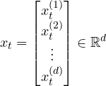$\begin{equation*} x_t= \begin{bmatrix} x_t^{(1)}\\ x_t^{(2)}\\ \vdots\\ x_t^{(d)} \end{bmatrix} \in\mathbb{R}^{d} \end{equation*}$

where

$d$ denotes the feature dimension,
$x_t^{(i)}$ denotes the $i^{\text{th}}$ feature measured at time step $t$ .

Equation (2.3) generalizes the scalar representation introduced in Equation (2.2). Throughout this article, every observation is represented as a column vector of dimension $d\times1$ . This convention is widely adopted in linear systems, control theory, and State Space Models, and it naturally extends to modern architectures such as S4 and Mamba.

Equation (2.4) is a specific instance of the general feature-vector representation defined in Equation (2.3). Each element of the vector corresponds to one physiological variable measured at the same instant.

Sequence Matrix Representation

A complete sequence is obtained by collecting observations over $T$ time steps. Since every observation $x_t$ is represented as a $d\times1$ column vector, the complete sequence is formed by concatenating these vectors along the temporal dimension,

(2.5) $\begin{equation*} X= \begin{bmatrix} x_1 & x_2 & \cdots & x_T \end{bmatrix} \in\mathbb{R}^{d\times T} \end{equation*}$

where the $t^{\text{th}}$ column of $X$ corresponds to the observation recorded at time step $t$ .

In Equation (2.5),

each column represents one observation in the sequence,
each row represents one feature measured across all time steps,
$d$ denotes the feature dimension, and
$T$ denotes the sequence length.

This representation is commonly used in linear dynamical systems, signal processing, and State Space Models because it naturally preserves the temporal ordering of observations while maintaining each observation as a column vector.

2.3 Order Preserves Information

The defining characteristic of sequential data is that the ordering of observations carries meaningful information. Unlike sets, where the arrangement of elements is irrelevant, exchanging the positions of observations in a sequence generally changes its interpretation. Consequently, sequence models must preserve temporal ordering while processing the data.

The importance of temporal ordering extends far beyond natural language and financial time series.

In speech recognition, changing the order of acoustic frames produces an entirely different spoken utterance.
In video understanding, shuffling image frames destroys the motion information required for activity recognition.
In electrocardiogram (ECG) analysis, rearranging cardiac cycles changes the morphology of the signal and may completely alter the clinical diagnosis.
In genomics, modifying the ordering of nucleotides changes the encoded biological information.

These examples demonstrate that the temporal arrangement of observations is an integral part of the information contained within a sequence. Consequently, an effective sequence model must preserve the order of observations throughout the learning process rather than treating them as independent samples.

This requirement distinguishes sequence models from conventional feedforward neural networks. While a feedforward network processes each input independently, a sequence model must continuously incorporate information from previous observations while processing the current one. As a result, sequence modeling requires mechanisms capable of retaining historical information, a concept that naturally leads to temporal dependency and the notion of memory, which are discussed in the following sections.

2.4 Temporal Dependency

A second defining characteristic of sequential data is that observations are not statistically independent. Instead, the current observation is often influenced by one or more previous observations. This dependence on historical information is known as temporal dependency.

In conventional machine learning, samples are assumed to be independently generated. Consequently, the probability of observing one sample is unaffected by the presence or absence of other samples. However, this assumption does not hold for sequential data, where the current observation is conditioned on the history of previous observations.

Mathematically, the probability of observing $x_t$ is expressed as

(2.6) $\begin{equation*} P(x_t)=P(x_t\mid x_1,x_2,\ldots,x_{t-1}) \end{equation*}$

Equation (2.6) states that the probability of the current observation depends on all previously observed inputs. In other words, the sequence possesses memory, and every new observation is interpreted in the context of the preceding observations.

More generally, the probability of observing an entire sequence $X$ can be factorized using the chain rule of probability as

(2.7) $\begin{equation*} P(X)=P(x_1,x_2,\ldots,x_T)= \prod_{t=1}^{T} P(x_t\mid x_1,x_2,\ldots,x_{t-1}). \end{equation*}$

Equation (2.7) is one of the fundamental equations in sequence modeling. It shows that modeling a sequence is equivalent to modeling a series of conditional probability distributions. Nearly all modern sequence models—including Recurrent Neural Networks (RNNs), Long Short-Term Memory (LSTM) networks, Gated Recurrent Units (GRUs), Transformers, and State Space Models (SSMs)—can be interpreted as different approaches for approximating these conditional probabilities.

The importance of temporal dependency is readily observed in natural language processing. Consider the partial sentence

The cat sat on the

The next word is not selected uniformly from the vocabulary. Instead, the probability distribution strongly favors semantically meaningful words such as mat, floor, or chair, while assigning very low probability to unrelated words.

Mathematically,

(2.8) $\begin{equation*} P(\text{mat}\mid\text{The cat sat on the}) \gg P(\text{banana}\mid\text{The cat sat on the}). \end{equation*}$

The model therefore predicts the next word by utilizing the contextual information contained in the preceding words.

A similar dependency exists in time-series forecasting. Let $p_t$ denote the stock price at time step $t$ . The future price depends on historical market behavior and is commonly represented as

(2.9) $\begin{equation*} P(p_t)= P(p_t\mid p_1,p_2,\ldots,p_{t-1}). \end{equation*}$

Likewise, in biomedical signal analysis, the interpretation of an ECG waveform depends not only on the current cardiac cycle but also on previous cycles. Detecting arrhythmias, estimating heart-rate variability, or identifying transient abnormalities requires analyzing the temporal evolution of the signal rather than isolated measurements.

The same principle applies across numerous applications.

In speech recognition, the pronunciation of the current phoneme depends on neighboring phonemes.
In video understanding, the interpretation of the current frame depends on preceding frames that describe the motion of objects.
In robotics, the current sensor measurements depend on the previous states of the robot.
In genomics, the biological function of a nucleotide often depends on the surrounding nucleotide sequence.

These examples illustrate that sequential observations are inherently correlated across time. Consequently, a sequence model cannot make accurate predictions by processing each observation independently.

Instead, it must retain information about previously observed inputs while continuously incorporating new observations. The challenge therefore is not only to process the current observation $x_t$ , but also to summarize all previously observed information in a compact and computationally efficient manner.

This requirement naturally leads to the concept of an internal state, also referred to as memory, which serves as a compressed representation of the sequence history. Rather than storing every past observation explicitly, the model continuously updates this state as new observations arrive. The concept of memory forms the mathematical foundation of Recurrent Neural Networks, Linear RNNs, State Space Models, Structured State Space Models (S4), and Selective State Space Models (Mamba), and is introduced in the next section.

Next will be:

In the next section, we introduce the concept of memory (state) as a compact representation of sequence history. We will discuss:

Why sequence models require memory
Memory as a recursive state representation
General state-update equations
How this formulation naturally leads to Recurrent Neural Networks (RNNs), Linear RNNs, State Space Models (SSMs), Structured State Space Models (S4), and Selective State Space Models (Mamba).

From RNNs to Mamba: A Mathematical Journey Through Modern Sequence Models: Part 1

1. Introduction

2. Understanding Sequential Data

2.1 Examples of Sequential Data

2.2 Mathematical Representation of a Sequence

Univariate Sequences

Multivariate Sequences

Sequence Matrix Representation

2.3 Order Preserves Information

2.4 Temporal Dependency

Next will be:

Leave a Reply Cancel reply

1. Introduction

2. Understanding Sequential Data

2.1 Examples of Sequential Data

2.2 Mathematical Representation of a Sequence

Univariate Sequences

Multivariate Sequences

Sequence Matrix Representation

2.3 Order Preserves Information

2.4 Temporal Dependency

Next will be:

Please Share This Share this content

You Might Also Like

Improved Interpretability and Explainability of Deep Learning Models

Quantum Computing Part 1

Exploring Single-Qubit and Multi-Qubit States with Qiskit

Leave a Reply Cancel reply

Share this content